Calculate and Plot Activity

Given an existing database for Al-Zn, we would like to calculate the activity of the liquid.

Experimental activity results

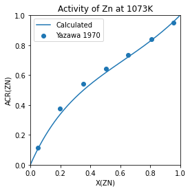
In order to make sure we are correct, we’ll compare the values with experimental results. Experimental activities are digitized from Fig. 18 in A. Yazawa, Y.K. Lee, Thermodynamic Studies of the Liquid Aluminum Alloy Systems, Trans. Japan Inst. Met. 11 (1970) 411–418.

The measurements at at 1073 K and they used a reference state of the pure Zn at that temperature.

exp_x_zn =   [0.0482, 0.1990, 0.3550, 0.5045, 0.6549, 0.8070, 0.9569]
exp_acr_zn = [0.1154, 0.3765, 0.5411, 0.6433, 0.7352, 0.8384, 0.9531]

Set up the database

Al-Zn database is taken from S. Mey, Reevaluation of the Al-Zn system, Zeitschrift Für Met. 84(7) (1993) 451–455.

from pycalphad import Database, equilibrium, variables as v
import numpy as np

dbf = Database('alzn_mey.tdb')

comps = ['AL', 'ZN', 'VA']
phases = list(dbf.phases.keys())

Calculate the reference state

Because all chemical activities must be specified with a reference state, we’re going to choose a reference state as the pure element at the same temperature, consistent with the experimental data.

components = ['ZN']
temperature = 1073
conditions = {v.N: 1, v.P: 101325, v.T: temperature}
ref_eq = equilibrium(dbf, components, phases, conditions)

Calculate the equilibria

Do the calculation over the composition range

conditions2 = {v.N: 1, v.P: 1013325, v.T: temperature, v.X('ZN'): (0, 1, 0.005)}
eq = equilibrium(dbf, comps, phases, conditions2)

Get the chemical potentials and calculate activity

We need to select the chemical potentials from the xarray Dataset and calculate the activity.

chempot_ref = ref_eq.MU.sel(component='ZN').squeeze()
chempot = eq.MU.sel(component='ZN').squeeze()

R = float(v.R)
acr_zn = np.exp((chempot - chempot_ref)/(R*temperature))

Plot the result

import matplotlib.pyplot as plt

plt.plot(eq.X.sel(component='ZN', vertex=0).squeeze(), acr_zn, label='Calculated', color='blue')

# add experimental data
plt.scatter(exp_x_zn, exp_acr_zn, label='Yazawa & Lee, 1970', color='red')

plt.xlim((0, 1))
plt.ylim((0, 1))
plt.gca().set_aspect(1)
plt.gcf().set_size_inches(9, 6)
plt.gcf().set_dpi(150)
plt.xlabel('X(Zn)')
plt.ylabel('ACR(Zn)')
plt.title(f'Activity of Zn at {temperature} K')
plt.legend(loc=0)

<matplotlib.legend.Legend at 0x12cbe7230>